Quantization 101!

Common data types used in machine learning

The size of a model is determined by the number of parameters and their precision in it. Floating point 32 bit (FP32) is a standard for representing real numbers in binary. It breaks down number into three parts - the sign, the exponent and the mantissa (significand).

Sign:

It indicates whether a number is positive or negative. Value of 0 represents a positive number while the value of 1 represents a negative number. 1 bit is assigned for the sign.

Exponent:

It determines the range of the number. It acts like power of 2 in scientific notation, scaling the mantissa. 8 bits are assigned to it and thus it can represent values from 0 to 255.

Mantissa:

It represents the precision of the number. It is the fractional part of the number which holds the significant digits.

Float32 (FP32):

Sign - 1 bit
Exponent - 8 bits
Mantissa - 23 bits

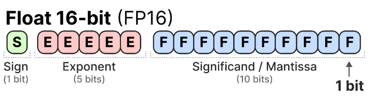
Float16 (FP16):

Sign - 1 bit
Exponent - 5 bits
Mantissa - 10 bits

FP16

You can see clearly the range of FP16 numbers is much smaller as compared to the range of FP32 making it prone to the risk of overflowing and underflowing. If you want to do a 10k * 10k operation you will end up with 100M which is not possible to represent since the max that can be represented using this representation is 64k.

BF16:

This was created to overcome the above problems. In this 8 bits are reserved for the exponent and 7 are for the fraction. Thus we can store more numbers but with less precision with respect to FP16.

In machine learning, FP32 is called as the full precision (4 bytes) while BF16 and FP16 are called as half precision (2 bytes).

So what to use? On one hand you have a full precision approach that has high precision but can store less information and then you have the half precision approach that is not prone to problems like overflowing and underflowing but can cause problems when it comes to precision.

So that is why we use a mixed precisoin approach where the model weights are held in FP32 while the computation of forward and backward pass are done for FP16/BF16 to enhance the training speed.

Explaining the above paragraph:

Training using full precision:

Now during the training of the model it is constantly learning and updating weights and this process relies entirely on gradient descent where small gradients are used to change the weights in the right direction- minimizing the loss! These gradients are extremely small and if we use a data type like that of FP16 these small values might get rounded up to 0 and the updating of the weights will stop and thus eventually the model will stop training.

Inference using half precision:

After the complete training of the model it is ready for inference, that is making predictions on new data. During this we just need to perform a forward pass and there is no updating of the model weights and the use of gradients and hence the precision requirement is much lower as compared to the training part.

Model Quantization:

The below details are inspired from this blog

What is quantization:

It is a process that reduces the number of bits that are required to represent a number. In machine learning it is used to convert a highly precise data type like FP32 to a low precision format like FP16 which reduces the size and increases the computational speed.

How it works?:

It maps a larger range of values from a high precision data type to a smaller one, low precision data type.

So let us say we have two data types: dt1 with values [0,1,2,3,4,5] and dt2 with values [0,2,4]. Let our vector be [3,1,2,3]

Step 1: Normalization: First we need to normalize our values in the source vector within a range which is typically between 0 and 1 or -1 and 1. This can be achieved by dividing all the values by the maximum value in the given vector:
- Original Vector : [3,1,2,3]
- Absolute Maximum : 3
- Normalized Vector : [3/3, 1/3, 2/3, 3/3] = [1.0, 0.33, 0.66, 1.0]
Step 2 : Scaling: Now we will scale our normalized values to an range of our target data type. The target data type dt2 has the range of 4 thus we can multiply our normalized vector by 4 to get the scaled vector.
- Normalized Vector : [1.0, 0.33, 0.66, 1.0]
- Target range : 4
- Scaled vector : [14, 0.334, 0.664, 1.04] = [4.0, 1.33, 2.66, 4.0]
Step 3 : Rounding
- 4.0 is rounded to 4.
- 1.33 is rounded to 0 (the nearest value in [0,2,4])
- 2.66 is rounded to 2.
- 4.0 is rounded to 4.

Thus the quantized vector is [4, 0, 2, 4]

Dequantization and Quantization Error:

To get the original numbers back we dequantize it by reversing the process: dividing by the target ranges and multiplying by the original maximum value.

Quantized vector : [4, 0, 2, 4]
Divided by the target range : [4/4, 0/4, 2/4, 4/4] = [1.0,, 0.0, 0.5, 1.0]
Multiplied by the original maximum value: [1.03, 0.03, 0.53, 1.03] = [3.0, 0.0, 1.5, 3.0]
Rounded to the nearest integer : [3, 0, 2, 3]

Note: The second element changes from 1 to 0, this is the quantization error. This is the information that is lost while we move from high precision to low precision. It is the same error that keeps on accumulating and potentially degrades model's overall performance.

How to make these methods more precise?

Strategy 1: Use a more specific "shrinking rule": The whole point of quantization is that we need to take a wide range of precise numbers and squish them into a small set of simple integers.

A very imprecise way will be to use one shrinking rule for everything. Let us say we have two groups of numbers

Group A : [30, 10, 20, 30] Group B : [0, 2, 2, 0]

As you can clearly observe A has large numbers as compared to the ones present in B. An imprecise shrinking rule will use a single shrinking rule for both groups based on the biggest number overall which 30. The rule might be "divide all the numbers of all groups by 4".

Group A becomes : [7.5, 2.5, 5, 7.5] -> Rounded to [8, 3, 5, 8] (Looks okay)
Group B becomes [0, 0.5, 0.5, 0] -> Rounded to [0, 1, 1, 0] (We lost some detail, 0.5 got rounded up)

So are you able to observe that this shrinking is quite aggressive for Group B? Why you ask? Because we over compressed values that were already small to begin with!

The solution! : Custom Rule for Each Group This method is called as "vector-wise quantization".

For Group A: [30, 10, 20, 30], the biggest number is 30. We can use a custom rule like "divide by 4".
For Group B: [0, 2, 2, 0], the biggest number is just 2. We can use a much gentler rule, like "divide by 1" (or don't shrink it at all!).

Thus the first way to improve precision is to stop using a global shrinking rule and start using specific rules so that we are able to shrink the given vector accordingly, there is no over or under shrinking of the values.

Strategy 2 : Isolate and Handle Extreme Outliers (Mixed Precision): Sometimes due to presence of an outlier (a values that is extremely different as compared to its peers in a vector) can cause the custom shirking rule to fail as well and thus we might lose all information.

The Solution: Handle the Outlier Separately

Isolate the outlier : First identify the outlier in your vector and pull it out.
Process in Two Parts:
- For the normal values of the vector use a gentle shrinking rule that is perfect according to their size.
- For the outlier number, depending upon its value you use a method that can handle its large/small size.

The above is an example of "Mixed Precision" since you are using both low and high level precision for the normal and the outlier values of the vector respectively in order to deal with this problem.

Strategy 3 : Advanced Calibration Methods :

Reasons why the custom shrinking rules of are not reliable"

1. Non-uniform distributions : Neural network weights and activations are non uniformly distributed and a simple custom rule often assumes the distribution to be either compress values too much or ignore rare but important outliers which leads to very large errors.
1. Layer sensitivity: Different layers have different ranges and using the same rule across all the layers can cause some layers to over quantized (losing important info) and some under quantized (wasting precision).

Now how do we find the best shrinking factor for each group of vectors? Like how do we choose whether to divided by 4 or by 3.8?

To solve this calibration comes into play.

Now how to select the range?

For this we will explore some of the basic calibration methods!

1. Min-Max Calibration:

scale = \frac{max - min}{2^{bits} - 1}

Example :

We have the vector:

x = [- 0.2, 0.1, 0.3, 0.5]

Compute the minimum and maximum:

min = - 0.2, max = 0.5

Compute the quantization scale:

scale = \frac{max - min}{255} = \frac{0.5 - (- 0.2)}{255} \approx 0.00275

Finally, convert to int8:

x_{int8} = round (\frac{x - min}{scale})

1. Percentile Calibration: The main idea is to ignore the extreme values using percentiles

Example:

We have the vector:

x = [- 0.2, 0.1, 0.3, 5.0]

Compute the 1st and 99th percentiles to reduce the effect of outliers:

1st percentile \approx - 0.2, 99th percentile \approx 0.3

Compute the quantization scale:

scale = \frac{0.3 - (- 0.2)}{255} \approx 0.0020

Clip the values to the percentile range and convert to int8:

x_{int8} = round (\frac{clip (x, - 0.2, 0.3) - (- 0.2)}{scale})

Why this over the Min-Max method? Well if there is presence of extreme outliers then the range becomes huge using the min-max method because of which the numbers might get compressed into a tiny part and we might lose precision.

The percentile method uses 1st and 99ht percentiles and because of this we are able to ignore the extreme outliers and focus on the part where most of the data lives

Using clip(x,-0.2,0.3), the x stays between the two percentile values only. If x is between -0.2 and 0.3 then it remains the same and if it is out of the range then it either becomes -0.2 ( if less than -0.2) or it becomes 0.3 (if greater than 0.3).

1. KL Divergence Calibration: So the core idea is very simple. We pick a range that minimizes the info loss between the original and the quantized distributions.

Example:

x = [0.1, 0.15, 0.2, 5.0]

We will try to quantize the above vector using multiple threshold values and then compute the KL divergence between the original histogram and the quantized histogram and then choose the threshold value with the lowest divergence of all.

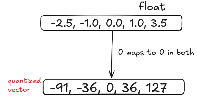
1. Symmetric and Asymmetric Quantization In symmetric quantization the range of numbers are kept symmetric around zero. This is done by using the absolute value of the max integer of the vector as the min and max.

How to do it?

Symmetric Quantization

Consider the following vector:
[-2.5, -1.0, 0.0, 1.0, 3.5]

Step 1: Find the max absolute value
max(|-2.5|, |3.5|) = 3.5
Step 2: Calculate the scale

S = \frac{max_abs}{127} = \frac{3.5}{127} = 0.02756

Step 3 : Zero point For symmetric quantization the zero point is fixed at 0 so we do not need to calculate it.
Step 4 : Quantize each element x by: $$ q = \text{round}\left(\frac{x}{S}\right) $$

After doing it the final quantized values will be as follows:

Quantized q = [-91, -36, 0, 36, 127]

Symmetric Quantization

Asymmetric Quantization

It is not symmetric around 0 and it maps the max and the min values from the given range of values to the quantized range.

Step 1 : Find the min and max of the original vector

min = -2.5 max = 3.5

Step 2 : Calculate the scale

S = \frac{max - min}{255} = \frac{3.5 - (- 2.5)}{255} = \frac{6.0}{255} = 0.02353

Step 3 : Calculate the zero point Z:

z = round (\frac{- (- 2.5)}{0.02353}) = round (\frac{2.5}{0.02353}) \approx round (106.2) = 106

Step 4 : Quantize each element x by:

q = round (\frac{x}{S} + Z)

SO the final vector will look like :

Quantized q = [0, 63, 106, 149, 255]

Asymmetric Quantization

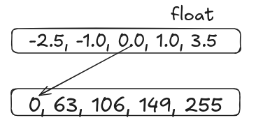
Here we can see that the zero point shift happens because the floating point range is not centered around zero and the quantized integer range has a fixed lower and upper bound.

Why do we need to calculate the zero point? Imagine you have a ruler that goes from -10 to +10. Normally, you'd assume your data is nicely centered around 0, so every marking on the ruler gets used efficiently.

But what if your data isn’t centered? Let’s say it actually ranges from +3 to +10. Suddenly, the portion of the ruler from -10 to +3 is wasted — all those markings are useless!

Asymmetric quantization solves this problem. It’s like sliding the ruler so that it starts exactly at your data’s minimum (+3) and ends at the maximum (+10). Now every single marking is meaningful, and we can represent our numbers more efficiently.

In short: the zero point tells us where to “anchor” our ruler so that no space is wasted and every integer truly counts.

References