Engineering Fully Local Retrieval-Augmented Generation Systems
The Paradigm of Localized Retrieval-Augmented Generation
Let's first understand what is parametric memory and non-parametric memory.
Parametric Memory: It is the memory that is stored in model's parameters during pre-training or fine-tuning. Traditional LLMs rely exclusively on parametric memory—the knowledge encoded within the model's weights during pre-training. While vast, this memory is static, prone to "hallucinations" (factually incorrect generations), and computationally expensive to update.
Non-Parametric Memory:This is knowledge stored outside the model, usually in vector databases (FAISS), document stores, knowledge graphs etc.
RAG augments this parametric memory with non-parametric memory!
RAG adds another layer of memory on top of what the model already knows. This new layer is non-parametric memory — basically an external, searchable database where all your real facts live.
During inference, RAG looks into this database, pulls out the most relevant pieces of information, and then slips them into the model’s prompt. Because of this, the model isn’t just guessing, it’s grounding its answer in actual, verifiable data.
This setup creates a clean separation of duties: the model handles the reasoning and writing part,while the retrieval system takes care of storing information and fetching the right pieces whenever needed.
Local RAG
Why local RAG? When all the processes of ingestion, embedding, retrieval, and generation run on your own machine or server, you unlock three huge advantages that cloud-based RAG simply can’t match.
- Your data stays yours (Privacy + Sovereignty)
If you're dealing with things like internal financial reports, unpublished research, or anything remotely confidential, sending that data to external APIs is a big no-go. With Local RAG, nothing leaves your system. Everything stays inside your own encrypted environment, giving you full control and zero exposure.
- No lag. No outages. No “retry later.” (Latency + Reliability)
Relying on cloud services means relying on the network—latency spikes, dropped connections, or random service outages. When everything runs locally, your response time is limited only by your hardware. It’s predictable, stable, and consistent.
- Costs stop scaling with tokens (Cost Predictability)
API-based RAG becomes expensive fast because you're billed for every token sent or generated. Local models flip this: you pay once for hardware or a fixed cloud instance, and you can run as many queries as you want. For high-volume or budget-sensitive applications, this is a game changer.
Understanding the basic framework - Transformers, Vectors and Quantization.
Before you can build a serious, fully local RAG pipeline, you need to understand the math and the architecture behind each component.
Attention is All You Need
The Transformer fundamentally changed deep learning by removing recurrence (RNNs/LSTMs) and replacing it with pure attention. Instead of processing tokens one-by-one, Transformers look at all tokens at once and learn global relationships.
The core operation of your RAG system should be to retrieve accurately Scaled Dot-Product Attention:
Vector Space Semantics
So retrieval in RAG works by converting your text chunks into vectors in a high dimensional space. For our project we will use all-MiniLM-L6-v2 model that uses Sentence-BERT (SBERT), which takes BERT and restructures it into a siamese network to produce sentence-level embeddings that actually reflect semantic similarity.
Sentence BERT 101: Let us go through the differences between BERT and Sentence BERT and understand what is what! BERT is trained using Masked Language Modeling (MLM) and Next Sentence Prediction (NSP). It’s great at token-level understanding, classification, and QA tasks. But here’s the catch: BERT outputs a vector for every token, plus a [CLS] token. The [CLS] embedding is not trained to represent the meaning of a full sentence. Because of that, cosine similarity between two BERT [CLS] vectors is basically meaningless.
Sentence-BERT: What Changes? SBERT starts from BERT (or RoBERTa, etc.) but introduces two critical improvements:
- A pooling layer
Instead of relying on the raw [CLS] token, SBERT does:
Mean pooling,max pooling or specially learned pooling. This produces a single fixed-size embedding for the entire sentence.
- Fine-tuning for similarity
SBERT is trained on sentence pairs using: Contrastive loss and triplet loss.
With the help of all of these techniques, semantically similar sentences end up close together, and unrelated ones move farther apart in vector space.
So the difference becomes simple:
BERT just understands sentences while SBERT understands as well as arranges sentences into a geometry where distances actually mean something
Why the Siamese Architecture Matters?
SBERT uses a siamese network: two or more identical encoder branches with shared weights. Each sentence in a training pair flows through its own path.
The training objectives enforce:
Positive pairs: pull embeddings closer
Negative pairs: push embeddings apart
This directly teaches the model that cosine similarity ≈ semantic similarity and that is exactly what nearest-neighbor retrieval needs.
Another big advantage: At inference time, you only encode a sentence once. After that, you compare embeddings using cheap vector operations—no need to run BERT cross-attention over every document.
Why SBERT is a better option for RAG?
For RAG systems we need embeddings that are stable, well-spread and most importantly semantically meaningful. SBERT does all of that. Also while using SBERT the process is computationally efficient for large corpora as you embed documents once, store them, and retrieval is just fast similarity search, not repeated cross‑attention between query and every document.
Normal BERT on the other hand suffer from issues like:
- Anisotropy (embeddings clump into a narrow cone in vector space).
- Randomly unrelated sentences often look too similar in cosine space.
Quantization and Model Compression:
Running LLMs on constrained hardware necessitates quantization - reducing the precision of the model's weights from standard floating-point formats to lower-bit representations.
In this project we will implement NF4 (Normal Float 4), a data type introduced by the QLoRA research. NF4 is information-theoretically optimal for weights normally distributed around zero, which is typical for neural networks.
Data Ingestion:
The adage "Garbage In, Garbage Out" is axiomatic in RAG. A RAG system retrieves from an external knowledge base; if that knowledge base is outdated, inconsistent, poorly chunked, or irrelevant, the retrieved context will mislead the LLM, causing wrong or hallucinated answers. Even with a strong retriever and powerful LLM, feeding it “garbage” (bad documents, bad chunking, missing key sources) yields “garbage” answers, because RAG does not create new ground truth—it amplifies whatever is in the underlying data.
For this project we are using a PDF. So, there is a problem.
How PDFs store data, a high level understanding: Each page has a “content stream” that is essentially a mini graphics program: “set font F, size 12; move to (x, y); draw text ‘Hello’; draw line here; place image there,” etc. Text is usually just glyphs placed at coordinates, not a continuous string with natural reading order.
So the PDF’s primary goal is: “given this file, any conforming viewer can render the same visual page,” not “given this file, a program can easily recover clean, ordered text with semantics.”
The code will deal with on how we will use the PDF of "Attention Is All You Need" research paper as a source for data ingestion.
Semantic Segmentation - its time to chunk
After extracting the linear stream of texts we need to segment them into discrete units (chunks). The model that we are using in this project "all-MiniLM-L6-v2" has a max sequence length of 256 tokens so if pass the entirety of the words we will face the problem of truncation because of which 90% of our information will be disregarded.
Some of the chunking strategies used are as follows:
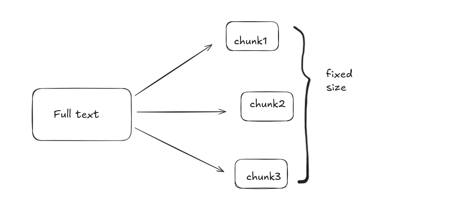
- Fixed Size: Split text into equal-sized segments (for example, 500 characters or 256 tokens), regardless of semantics.
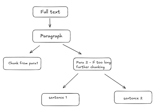
- Recursive Character Splitting: Split text hierarchically, first by paragraphs, then by sentences, then by characters, until chunks fit within a size limit.
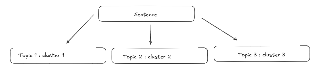
- Semantic Chunking: Use embeddings to segment text by topic similarity. Adjacent sentences that are semantically close are grouped.
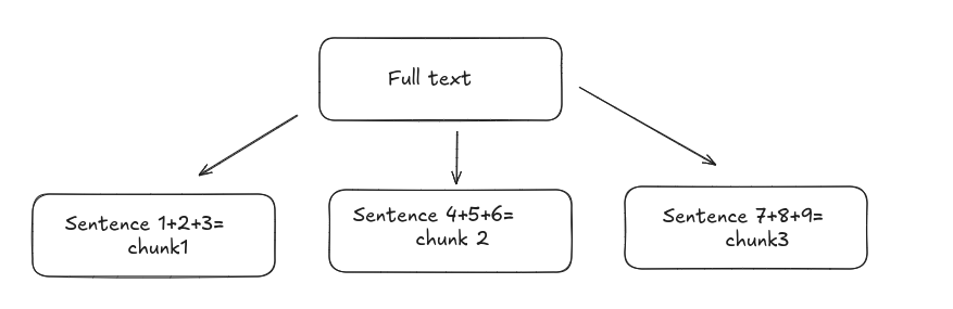
Language Based Chunking: Split text using linguistic boundaries (sentences, paragraphs). Tools like spaCy, NLTK, or Hugging Face tokenizers are common to be used.
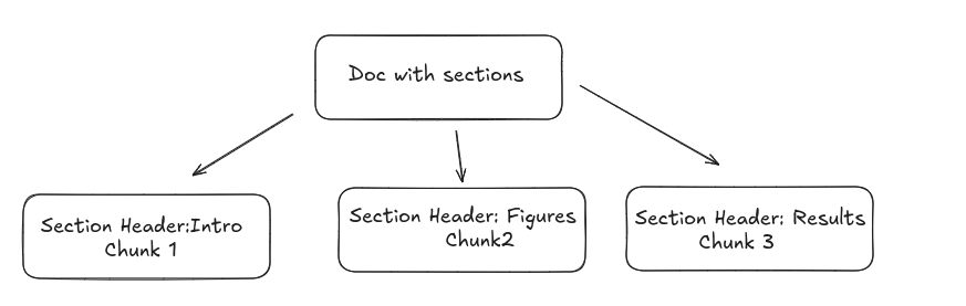
Context Aware Chunking: Context-aware chunking is an adaptive method for splitting documents into chunks that preserves meaningful structure and context, rather than just breaking text at fixed intervals. It uses document structure (like section headers), metadata (such as author or date), and domain-specific rules (for example, keeping entire code functions together) to create chunks that are more semantically coherent and useful for downstream tasks like retrieval in a RAG system.
The industry standard for processing prose and academic text is the Recursive Character Text Splitter.
So for the same reasons we will be using the recursive character text splitting in this project.
Read more about the techniques of chunking (here)
Chunk Size and Overlap
When you’re preparing long documents for a RAG system, you can’t just feed them in as a single block. You need to break the text into smaller, meaningful pieces—chunks—so they can be embedded, stored, and retrieved efficiently. Two hyperparameters control how this splitting works: chunk size and chunk overlap.
Chunk Size: Chunk size defines how big each chunk is. You usually measure it in:
characters (e.g., 500–1000 characters), or
tokens (e.g., 200–300 tokens)
Larger chunk size means we will able to capture more context but there will be less precision and smaller chunk size will allow us to capture less context but with more precision. So at the end of the day it is a trade-off between precision and capturing the context of the documents.
Chunk Overlap: Chunk overlap defines how much text is shared between consecutive chunks. It’s measured in the same unit as chunk size (characters or tokens).
It is important as it prevents awkward boundary cuts by making sure that:sentences aren’t split right in the middle, definitions or formulas that span a boundary stay intact and both the retriever and the LLM see complete, coherent ideas.
Example (characters)
Chunk size = 1000, overlap = 200
Chunk 1 → characters 0–999
Chunk 2 → characters 800–1799
Chunk 3 → characters 1600–2599
Each new chunk repeats the last 200 characters of the previous one.
Why These Hyperparameters Matter for RAG??
Chunk size controls the trade-off between context and precision while the overlap guarantees continuity so the model doesn’t lose information at boundaries.
The usual strategy is simple:Pick a chunk size that fits comfortably within your embedding model’s token limit,then add a moderate overlap (around 10–30% of chunk size) to preserve context across boundaries. This combination gives you clean, self-contained chunks that retrieve well and ground the LLM’s answers reliably.
Vector Indexing and Retrieval System:
A RAG system is only as good as its retrieval layer. Once we’ve chunked the document, we need a way to turn each chunk into a vector, store those vectors efficiently, and quickly find the most relevant ones when the user asks a question. This is where embeddings, FAISS, and similarity search come into play.
Generating Embeddings:
To convert text into machine-understandable vectors, we use the sentence-transformers library with the model all-MiniLM-L6-v2. This model produces a 384-dimensional dense embedding for any given text.
FAISS Vector Database:
Once we’ve generated embeddings for every chunk in the document, we need a fast, reliable way to store and search them. For this, we use FAISS (Facebook AI Similarity Search)—the industry-standard library for vector search.
Working of FAISS:
Indexing: You add your precomputed vectors (e.g., from all-MiniLM) to a FAISS index, which organizes them for fast search.
Searching: When you want to find similar items, you pass a query vector to FAISS, and it returns the most similar vectors from the index, usually as a list of IDs and similarity scores.
Efficiency: FAISS uses advanced algorithms like k-means clustering, inverted files, and hierarchical navigable small world (HNSW) graphs to speed up searches, even on massive datasets.
Hardware optimization: It leverages multi-core CPUs and GPUs for parallel processing, reducing search time and latency
Various indexes provided by FAISS:
FAISS provides several types of indexes, each optimized for different trade-offs in dataset size, speed, accuracy, and memory usage. Some of them are IndexFlatL2, IndexFlatIP, IndexIVFFlat, IndexHNSW etc.
Usually for small datasets and for getting an exact search out of the corpus we use IndexFlatL2.
IndexFlatL2:“Flat” - no clustering, no approximation; FAISS stores all vectors as-is. Search method - brute-force computation of L2 (Euclidean) distance between the query vector and every vector in the index.
Using Phi-3-mini-4k-instruct for Local RAG
After retrieval, we need a lightweight, fast LLM for answering queries using the retrieved context.
A step by step implementation can be found (here)
Resources: